Multi-layer Perceptron and Backpropagation
Get familiar with the MLP for classification
This demonstration for MLP and Backpropagation:
- Create fake data that is non-linearly separable
- Build model with O1 hidden layer (total 2)
# To support both python 2 and python 3
from __future__ import division, print_function, unicode_literals
import math #mathematics
import numpy as np #for data handling
import matplotlib.pyplot as plt #for drawing
from google.colab import files #save and upload files
%matplotlib inline
Generate fake data
X, y with some non-linear relations, e.g.
$x_1 = r*sin(t)$,
$x_2 = r*cos(t) + random*0.2$
Labels: $y = 0, 1, 2$
# Task 1 is to generate 3 classes of 100 points in 2d
C = 3 # number of classes
N = 100
d0 = 2 # dimensionality - 2 rows


#create input matrix X:
X = np.zeros((d0, N*C))
print(X.shape)#create class labels
y = np.zeros(N*C, dtype='uint8') #can set the type for the array (real label = groud truth)

#generate X, y with some non-linear relations, e.g. x1 = r*sin(t), x2 = r*cos(t) + random*0.2
# y = 0, 1, 2

for j in range(C):
  ix = range(N*j, N*(j+1)) # 0->100->200->300 (3 intervals)
  r = np.linspace(0.0, 1, N) # radius (create array 0, 0.01, 0.02,....1)
  t = np.linspace(j*4, (j+1)*4, N) + np.random.randn(N) * 0.2
  #print(t.T.shape)
  X[:, ix] = np.c_[r*np.sin(t), r*np.cos(t)].T #concate and transpose (300, 2)-->(2, 300)
  y[ix] = j

print("y:\n", y, y.shape)
Visualization the shape
plt.scatter(X[:N, 0], X[:N, 1], c=y[:N], s=40, cmap=plt.cm.Spectral)
# plt.axis('off')
plt.xlim([-1.5, 1.5]) #Get or set the x limits of the current axes.
plt.ylim([-1.5, 1.5])
cur_axes = plt.gca() #Get the current Axes instance on the current figure matching the given keyword args, or create one.
cur_axes.axes.get_xaxis().set_ticks([])
cur_axes.axes.get_yaxis().set_ticks([])

plt.plot(X[0, :N], X[1, :N], 'bs', markersize = 7) #blue square 0-100
plt.plot(X[0, N:2*N], X[1, N:2*N], 'ro', markersize = 7) # red oval 100-200
plt.plot(X[0, 2*N:], X[1, 2*N:], 'g^', markersize = 7); # green triangle 200-300

plt.savefig('EX.png', bbox_inches='tight', dpi = 600)
plt.show()

Optional:
To download the image file, You need to add these two lines:
from google.colab import files
files.download('file.txt')
#files.download('EX.png')
Solution We want to separate the 3 class using a MLP. We plan to add a hidden layer between in/out while Softmax regression can only use for linear separation. Activation is ReLU: f(s) = max(s, 0), f'(s) = 0 if s ≤ 0, f'(s) = 1 otherwise.
It is benefitial for an activation function to be simple to get derivative.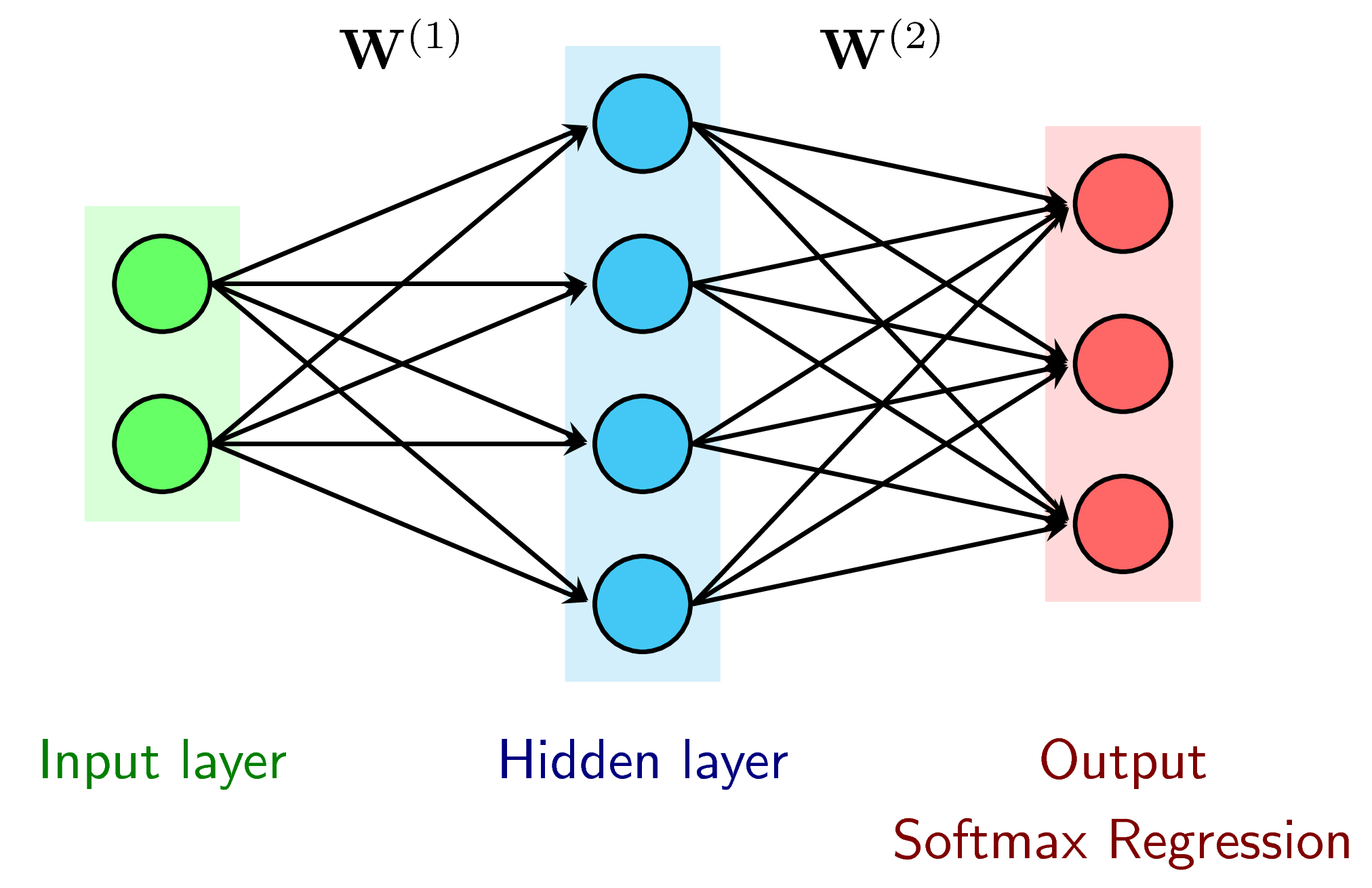
Feedforward
A1 ($l_0->l_1$) is Relu activation function. A2 = softmax ($l_1$-> output) $Z^{(i)}$ is the input of each layer
\begin{eqnarray} \mathbf{Z}^{(1)} &=& \mathbf{W}^{(1)T}\mathbf{X} \\ \mathbf{A}^{(1)} &=& \max(\mathbf{Z}^{(1)}, \mathbf{0}) \\ \mathbf{Z}^{(2)} &=& \mathbf{W}^{(2)T}\mathbf{A}^{(1)} \\ \mathbf{\hat{Y}} = \mathbf{A}^{(2)} &=& \text{softmax}(\mathbf{Z}^{(2)}) \end{eqnarray}Loss function (using cross-entropy)
$J \triangleq J(\mathbf{W, b}; \mathbf{X, Y}) = -\frac{1}{N}\sum_{i = 1}^N \sum_{j = 1}^C y_{ji}\log(\hat{y}_{ji})$
here, we added $\frac{1}{N}$ to avoid big sum with Batch Gradient Descent (BGD).
Backpropagation
Note: use derivative of softmax regression
\begin{eqnarray} \mathbf{E}^{(2)} &=& \frac{\partial J}{\partial \mathbf{Z}^{(2)}} =\frac{1}{N}(\mathbf{\hat{Y}} - \mathbf{Y}) \\ \frac{\partial J}{\partial \mathbf{W}^{(2)}} &=& \mathbf{A}^{(1)} \mathbf{E}^{(2)T} \\ \frac{\partial J}{\partial \mathbf{b}^{(2)}} &=& \sum_{n=1}^N\mathbf{e}_n^{(2)} \\ \mathbf{E}^{(1)} &=& \left(\mathbf{W}^{(2)}\mathbf{E}^{(2)}\right) \odot f’(\mathbf{Z}^{(1)}) \\ \frac{\partial J}{\partial \mathbf{W}^{(1)}} &=& \mathbf{A}^{(0)} \mathbf{E}^{(1)T} = \mathbf{X}\mathbf{E}^{(1)T}\\ \frac{\partial J}{\partial \mathbf{b}^{(1)}} &=& \sum_{n=1}^N\mathbf{e}_n^{(1)} \\ \end{eqnarray}#create some functions:
def softmax(V):
"""V is a vector Z is a vector of probability (0, 1)"""
e_V = np.exp(V - np.max(V, axis = 0, keepdims = True)) # MAX.keepdims.True, the axes which are reduced are left in the result as dimensions with size one.
sum = e_V.sum(axis = 0);
Z = e_V / sum
return Z
#One-hot coding: Categorical data a, b, c --> [100, 010, 001]
#coo_matrix((data, (row, col)), shape=(4, 4))
# >>> # Constructing a matrix using ijv format
#>>> row = np.array([0, 3, 1, 0])
#>>> col = np.array([0, 3, 1, 2])
#>>> data = np.array([4, 5, 7, 9])
#>>> coo_matrix((data, (row, col)), shape=(4, 4)).toarray()
#array([[4, 0, 9, 0],
# [0, 7, 0, 0],
# [0, 0, 0, 0],
# [0, 0, 0, 5]])
#one_likes: create a matrix of one like a given matrix (same sizes)
from scipy import sparse
def convert_labels(y, C = 3):
Y = sparse.coo_matrix((np.ones_like(y), (y, np.arange(len(y)))), shape = (C, len(y))).toarray()
return Y
# cost or loss function
def cost(Y, Yhat):
return -np.sum(Y*np.log(Yhat))/Y.shape[1]
The training implementation
d0 = 2
d1 = h = 100 # size of hidden layer
d2 = C = 3 # number of classes

iter = 5000 #number of training iteration

# initialize parameters randomly

W1 = 0.01*np.random.randn(d0, d1) # normal distribution weight 1 (layer) 2X100
b1 = np.zeros((d1, 1)) # bias 1

W2 = 0.01*np.random.randn(d1, d2) # 2nd layer: 100x 3
b2 = np.zeros((d2, 1)) #bias 2

#Both W1, W2 need to be optimized.

Y = convert_labels(y, C)
print("Y:\n", Y, Y.shape)
N = X.shape[1] #cols

eta = 1 # learning rate

for i in range(iter):
  #Feedforward:
  Z1 = np.dot(W1.T, X) + b1
  A1 = np.maximum(Z1, 0) #ReLU
  Z2 = np.dot(W2.T, A1)
  Yhat = softmax(Z2)

  # print loss after each 1000 iterations
  if (i % 1000 == 0):
    loss = cost(Y, Yhat)
    print("iter %d, loss: %f" %(i, loss))


  #Backpropagation
  E2 = (Yhat - Y)/N
  dW2 = np.dot(A1, E2.T) #f'(W2)
  db2 = np.sum(E2, axis = 1, keepdims = True) #f'(b2)

  E1 = np.dot(W2, E2)
  E1[Z1 <= 0] = 0 # assign all value < 0 to 0 (gradient of ReLU)
  dW1 = np.dot(X, E1.T)
  db1 = np.sum(E1, axis = 1, keepdims = True)

  #gradient descent update
  W1 += -eta*dW1
  b1 += -eta*db1
  W2 += -eta*dW2
  b2 += -eta*db2
#After training, we have W1, W2, b1, b2 ready. Now apply to get the input and output
Z1 = np.dot(W1.T, X) + b1
A1 = np.maximum(Z1, 0)
Z2 = np.dot(W2.T, A1) + b2
predicted_class = np.argmax(Z2, axis=0)
print('training accuracy: %.2f %%' % (100*np.mean(predicted_class == y)))
Visualize results
cmaps['Miscellaneous'] = [ 'flag', 'prism', 'ocean', 'gist_earth', 'terrain', 'gist_stern', 'gnuplot', 'gnuplot2', 'CMRmap', 'cubehelix', 'brg', 'gist_rainbow', 'rainbow', 'jet', 'nipy_spectral', 'gist_ncar']
#set up axis
xm = ym = np.arange(-1.5, 1.5, 0.025)
#xlen = ylen =  len(xm)

(xx, yy) = np.meshgrid(xm, ym) #120 *120
#print("xx:\n", xx,"yy\n", yy)
#print(xx == yy.T)

xx1 = xx.ravel().reshape(1, xx.size)
yy1 = yy.ravel().reshape(1, yy.size)

#new input X0
X0 = np.vstack((xx1, yy1))
print("xx1:\n", xx1,"\n", xx1.shape, "\nyy1:\n", yy1,"\n", yy1.shape, "\nX0:\n", X0, "\n Shape: \n", X0.shape)

#Copy from above now replace with X0
Z1 = np.dot(W1.T, X0) + b1
A1 = np.maximum(Z1, 0)
Z2 = np.dot(W2.T, A1) + b2
print("Z2:\n", Z2)
# predicted class of each X0
Z = np.argmax(Z2, axis=0)# index of max val in axis 0 (row)


Z = Z.reshape(xx.shape)
print("Z:", Z)
print(Z.shape)
CS = plt.contourf(xx, yy, Z, 200, cmap='jet', alpha = .1) #draw contour

# Draw old data
plt.plot(X[0, :N], X[1, :N], 'bs', markersize = 7) #blue square
plt.plot(X[0, N:2*N], X[1, N:2*N], 'g^', markersize = 7) #green triangle
plt.plot(X[0, 2*N:], X[1, 2*N:], 'ro', markersize = 7) # red oval

#remove axis
# plt.xlim([-1.5, 1.5])
# plt.ylim([-1.5, 1.5])
# cur_axes = plt.gca()
# cur_axes.axes.get_xaxis().set_ticks([])
# cur_axes.axes.get_yaxis().set_ticks([])

# plt.xlim(-1.5, 1.5)
# plt.ylim(-1.5, 1.5)
# plt.xticks(())
# plt.yticks(())
plt.title('#hidden units = %d, accuracy = %.2f %%' %(d1, 99.33))
#Save file
fn = 'ex_res'+ str(d1) + '.png'
plt.show()
