
As deep learning on graphs is trending recently, this article will quickly demonstrate how to use networkx to turn rating matrices, such as MovieLens dataset, into graph data.
The rating data
We use rating data from the movie lens. The rating data is loaded into rdata which is a Pandas DataFrame. This article demonstrates how to preprocess movie lens data.
After processing, the rdata should look like this:
| userId | movieId | rating | timestamp | |
|---|---|---|---|---|
| 0 | 196 | 242 | 3 | 881250949 |
| 1 | 186 | 302 | 3 | 891717742 |
| 2 | 22 | 377 | 1 | 878887116 |
| 3 | 244 | 51 | 2 | 880606923 |
| 4 | 166 | 346 | 1 | 886397596 |
Nevertheless, we should avoid confusion between userId and movieId. Therefore, we added the prefix for each id as follow.
rdata['userId'] = 'u' + rdata['userId'].astype(str)
rdata['movieId'] = 'i' + rdata['movieId'].astype(str)
rdata.head()| userId | movieId | rating | timestamp | |
|---|---|---|---|---|
| 0 | u196 | i242 | 3 | 881250949 |
| 1 | u186 | i302 | 3 | 891717742 |
| 2 | u22 | i377 | 1 | 878887116 |
| 3 | u244 | i51 | 2 | 880606923 |
| 4 | u166 | i346 | 1 | 886397596 |
Transform the matrix to a bipartite graph
We will use networkx to create a bipartite undirected weighted graph. It is simple as follows.
import networkx as nx
from networkx import *
#Create a graph
G = nx.Graph()
#Add nodes
G.add_nodes_from(rdata.userId, bipartite=0)
G.add_nodes_from(rdata.movieId, bipartite=1)
#Add weights for edges
G.add_weighted_edges_from([(uId, mId,rating) for (uId, mId, rating)
              in rdata[['userId', 'movieId', 'rating']].to_numpy()])
Get graph properties
First, we can get the basic information about the graph
print(info(G))
#Name: MovieLens Bipartite
#Type: Graph
#Number of nodes: 2625
#Number of edges: 100000
#Average degree:  76.1905
We now can check if the graph is directed, multi-graphs, or bipartite.
G.is_directed(), G.is_multigraph(), is_bipartite(G)
#(False, False, True)
Next, we can get a more detailed insight into this graph.
print("radius: %d" % radius(G))
#radius: 3
print("diameter: %d" % diameter(G))
#diameter: 5
print("eccentricity: %s" % eccentricity(G))
#eccentricity: {'u196': 4, 'u186': 4, 'u22': 4,...}
print("center: %s" % center(G))
#center: ['u6', 'u62', 'u286', 'u200', 'u303',...]
print("periphery: %s" % periphery(G))
#periphery: ['u50', 'u97', 'u284', 'u242',...]
print("density: %s" % density(G))
#density: 0.029036004645760744
Visualize the graph
For better visualization, we first map nodes with two colours:
color_map = []
for node in G.nodes:
  if str(node).startswith('u'):
    color_map.append('yellow')
  else:
    color_map.append('green')
After that, we use networkx to draw the graph, spring and bipartite.
pos = nx.spring_layout(G)
plt.figure(3,figsize=(12,12))
nx.draw(G,pos,node_color=color_map)
plt.show()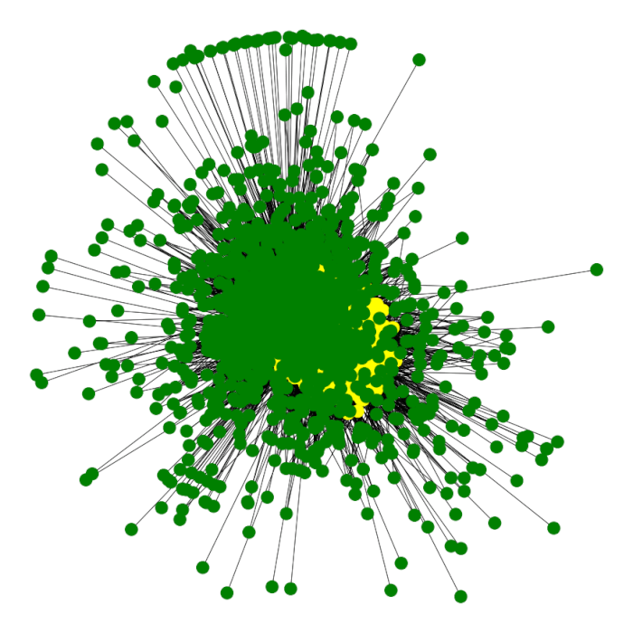
Otherwise, we can use the classical plot for bipartite graph as flow.
X, Y = bipartite.sets(G)
pos = dict()
pos.update( (n, (1, i)) for i, n in enumerate(X) ) # put nodes from X at x=1
pos.update( (n, (2, i)) for i, n in enumerate(Y) ) # put nodes from Y at x=2
nx.draw(G, pos=pos, node_color=color_map)
plt.show()
Now, the graph is ready for your learning algorithm.
