
The features you use influence more than everything else the result. No algorithm alone, to my knowledge, can supplement the information gain given by correct feature engineering.
What is a feature and why we need engineering of it? Basically, all machine learning algorithms use some input data to create outputs. This input data comprise features, which are usually in the form of structured columns. Algorithms require features with some specific characteristics to work properly. Thus, the need for feature engineering arises. Feature engineering efforts mainly have two goals:
- Preparing the proper input dataset, compatible with the machine learning algorithm requirements.
- Improving the performance of machine learning models.
According to a survey in Forbes, data scientists spend 80% of their time on data cleaning and preparation:

This metric is very impressive to show the importance of feature engineering in data science. Thus, we write this article to summarize the main techniques of feature engineering with their short descriptions. As it is hard to write an article for every method above, we try to keep the explanations brief and informative.
1.Imputation
Missing values are one of the most common problems when you try to prepare your data for machine learning. The reason for the missing values might be human errors, interruptions in the data flow, privacy concerns, and so on. Whatever is the reason, missing values affect the performance of the machine learning models.
Some machine learning platforms automatically drop the rows which include missing values in the model training phase. It can also decrease the model performance because of the reduced training size. On the other hand, most of the algorithms do not accept datasets with missing values and gives an error.
The most simple solution to the missing values is to drop the rows or the entire column. There is not an optimum threshold for dropping. However, you can use 70% as a thredhold to drop the rows and columns having higher missing values rate.
threshold = 0.7#Dropping columns with missing value rate higher than threshold
data = data[data.columns[data.isnull().mean() < threshold]]
#Dropping rows with missing value rate higher than threshold
data = data.loc[data.isnull().mean(axis=1) < threshold]
Numerical Imputation
Imputation is a more preferable option rather than dropping because it preserves the data size. However, there is an important selection of what you impute to the missing values. I suggest beginning with considering a possible default value of missing values in the column. For example, if a column only has 1 and NA, then it is likely that NA rows correspond to 0. Or if a column shows the “customer visit count in last month”, the missing values might be replaced with 0. As long as you think it is a sensible solution.
Another reason for the missing values is joining tables with different sizes and in this case, imputing 0 might be reasonable as well.
Except for the case of having a default value for missing values, I think the best imputation way is to use the medians of the columns. As the averages of the columns are sensitive to the outlier values, while medians are more solid in this respect.
#Filling all missing values with 0
data = data.fillna(0)#Filling missing values with medians of the columns
data = data.fillna(data.median())
Categorical Imputation
Replacing the missing values with the maximum occurred value in a column is a good option for handling categorical columns. But if you think the values in the column are distributed uniformly and there is not a dominant value, imputing a category like “Other” might be more sensible, because in such a case, your imputation is likely to converge a random selection.
#Max fill function for categorical columns
data['column_name'].fillna(data['column_name'].value_counts()
.idxmax(), inplace=True)
2.Handling Outliers
Before mentioning how outliers can be handled, I want to state that the best way to detect the outliers is to demonstrate the data visually. All other statistical methodologies are open to making mistakes, whereas visualizing the outliers gives a chance to take a decision with high precision. Anyway, I am planning to focus visualization deeply in another article and let’s continue with statistical methodologies.
Statistical methodologies are less precise as I mentioned, but on the other hand, they have a superiority, they are fast. Here I will list two different ways of handling outliers. These will detect them using standard deviation, and percentiles.
Outlier Detection with Standard Deviation
If a value has a distance to the average higher than x * standard deviation, it can be assumed as an outlier. Then what x should be?
There is no trivial solution for x, but usually, a value between 2 and 4 seems practical.
#Dropping the outlier rows with standard deviation
factor = 3
upper_lim = data['column'].mean () + data['column'].std () * factor
lower_lim = data['column'].mean () - data['column'].std () * factor
data = data[(data['column'] < upper_lim) & (data['column'] > lower_lim)]
In addition, z-score can be used instead of the formula above. Z-score (or standard score) standardizes the distance between a value and the mean using the standard deviation.
Outlier Detection with Percentiles
Another mathematical method to detect outliers is to use percentiles. You can assume a certain percentage of the value from the top or the bottom as an outlier. The key point is here to set the percentage value once again, and this depends on the distribution of your data as mentioned earlier.
Additionally, a common mistake is using the percentiles according to the range of the data. In other words, if your data ranges from 0 to 100, your top 5% is not the values between 96 and 100. Top 5% means here the values that are out of the 95th percentile of data.
#Dropping the outlier rows with Percentiles
upper_lim = data['column'].quantile(.95)
lower_lim = data['column'].quantile(.05)
data = data[(data['column'] < upper_lim) & (data['column'] > lower_lim)]
An Outlier Dilemma: Drop or Cap
Another option for handling outliers is to cap them instead of dropping. Capping keeps your data size and replace some values that meet condition with other values . At the end of the day, it might be better for the final model performance.
On the other hand, capping can affect the distribution of the data, thus it better not to exaggerate it.
#Capping the outlier rows with Percentiles
upper_lim = data['column'].quantile(.95)
lower_lim = data['column'].quantile(.05)data.loc[(df[column] > upper_lim),column] = upper_lim
data.loc[(df[column] < lower_lim),column] = lower_lim
3.Binning
Binning can be applied on both categorical and numerical data:
#Numerical Binning ExampleValue      Bin
0-30   ->  Low
31-70  ->  Mid
71-100 ->  High#Categorical Binning ExampleValue      Bin
Spain  ->  Europe
Italy  ->  Europe
Chile  ->  South America
Brazil ->  South America
The main motivation of binning is to make the model more robust and prevent overfitting, however, it has a cost to the performance. Every time you bin something, you sacrifice information and make your data more regularized.
The trade-off between performance and overfitting is the key point of the binning process. In my opinion, for numerical columns, except for some obvious overfitting cases, binning might be redundant for some kind of algorithms, due to its effect on model performance.
However, for categorical columns, the labels with low frequencies probably affect the robustness of statistical models negatively. Thus, assigning a general category to these less frequent values helps to keep the robustness of the model. For example, if your data size is 100,000 rows, it might be a good option to unite the labels with a count less than 100 to a new category like “Other”.
#Numerical Binning Exampledata['bin'] = pd.cut(data['value'], bins=[0,30,70,100], labels=["Low", "Mid", "High"])   value   bin
0      2   Low
1     45   Mid
2      7   Low
3     85  High
4     28   Low#Categorical Binning Example     Country
0      Spain
1      Chile
2  Australia
3      Italy
4     Brazilconditions = [
    data['Country'].str.contains('Spain'),
    data['Country'].str.contains('Italy'),
    data['Country'].str.contains('Chile'),
    data['Country'].str.contains('Brazil')]
choices = ['Europe', 'Europe', 'South America', 'South America']
data['Continent'] = np.select(conditions, choices, default='Other')     Country      Continent
0      Spain         Europe
1      Chile  South America
2  Australia          Other
3      Italy         Europe
4     Brazil  South America
4.Log Transform
Logarithm transformation (or log transform) is one of the most commonly used mathematical transformations in feature engineering. What are the benefits of log transform:
- It helps to handle skewed data and after transformation, the distribution becomes more approximate to normal.
- In most of the cases the magnitude order of the data changes within the range of the data. For instance, the difference between ages 15 and 20 is not equal to the ages 65 and 70. In terms of years, yes, they are identical, but for all other aspects, 5 years of difference in young ages mean a higher magnitude difference. This type of data comes from a multiplicative process and log transform normalizes the magnitude differences like that.
- It also decreases the effect of the outliers, due to the normalization of magnitude differences and the model become more robust.
A critical note: The data you apply log transform must have only positive values, otherwise you receive an error. Also, you can add 1 to your data before transform it. Thus, you ensure the output of the transformation to be positive.
Log(x+1)
#Log Transform Example
data = pd.DataFrame({'value':[2,45, -23, 85, 28, 2, 35, -12]})data['log+1'] = (data['value']+1).transform(np.log)#Negative Values Handling
#Note that the values are different
data['log'] = (data['value']-data['value'].min()+1) .transform(np.log)   value  log(x+1)  log(x-min(x)+1)
0      2   1.09861          3.25810
1     45   3.82864          4.23411
2    -23       nan          0.00000
3     85   4.45435          4.69135
4     28   3.36730          3.95124
5      2   1.09861          3.25810
6     35   3.58352          4.07754
7 -12 nan 2.484915.One-hot encoding
One-hot encoding is one of the most common encoding methods in machine learning. This method spreads the values in a column to multiple flag columns and assigns 0 or 1 to them. These binary values express the relationship between grouped and encoded column.
This method changes your categorical data, which is challenging to understand for algorithms, to a numerical format and enables you to group your categorical data without losing any information. (For details please see the last part of Categorical Column Grouping)
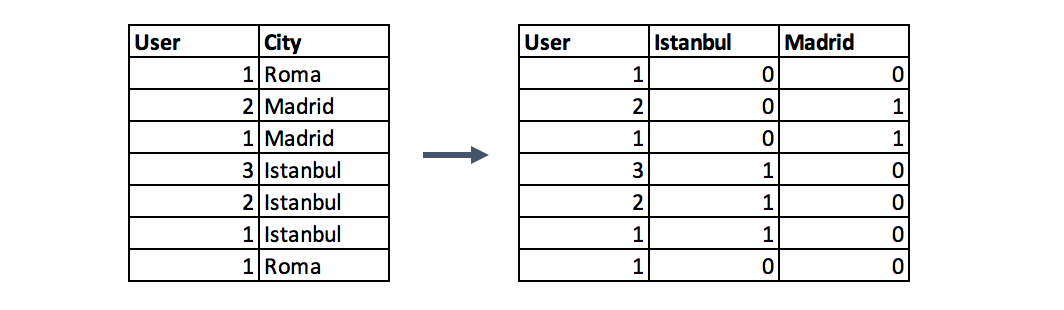
Why One-Hot?: If you have N distinct values in the column, it is enough to map them to N-1 binary columns, because the missing value can be deducted from other columns. If all the columns in our hand are equal to 0, the missing value must be equal to 1. This is the reason why it is called as one-hot encoding. However, I will give an example using the get_dummies function of Pandas. This function maps all values in a column to multiple columns.
encoded_columns = pd.get_dummies(data['column'])
data = data.join(encoded_columns).drop('column', axis=1)
6.Grouping Operations
In most machine learning algorithms, every instance is represented by a row in the training dataset, where every column show a different feature of the instance. This kind of data called “Tidy”.
Tidy datasets are easy to manipulate, model and visualise, and have a specific structure: each variable is a column, each observation is a row, and each type of observational unit is a table.
Datasets such as transactions rarely fit the definition of tidy data above, because of the multiple rows of an instance. In such a case, we group the data by the instances and then every instance is represented by only one row.
The key point of group by operations is to decide the aggregation functions of the features. For numerical features, average and sum functions are usually convenient options, whereas for categorical features it more complicated.
Categorical Column Grouping
I suggest three different ways for aggregating categorical columns:
- The first option is to select the label with the highest frequency. In other words, this is the max operation for categorical columns, but ordinary max functions generally do not return this value, you need to use a lambda function for this purpose.
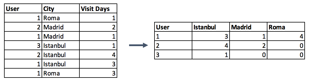
data.groupby('id').agg(lambda x: x.value_counts().index[0])- Second option is to make a pivot table. This approach resembles the encoding method in the preceding step with a difference. Instead of binary notation, it can be defined as aggregated functions for the values between grouped and encoded columns. This would be a good option if you aim to go beyond binary flag columns and merge multiple features into aggregated features, which are more informative.
#Pivot table Pandas Example
data.pivot_table(index='column_to_group', columns='column_to_encode', values='aggregation_column', aggfunc=np.sum, fill_value = 0)- Last categorical grouping option is to apply a group by function after applying one-hot encoding. This method preserves all the data -in the first option you lose some-, and in addition, you transform the encoded column from categorical to numerical in the meantime. You can check the next section for the explanation of numerical column grouping.
Numerical Column Grouping
Numerical columns are grouped using sum and mean functions in most of the cases. Both can be preferable according to the meaning of the feature. For example, if you want to obtain ratio columns, you can use the average of binary columns. In the same example, sum function can be used to obtain the total count either.
#sum_cols: List of columns to sum
#mean_cols: List of columns to averagegrouped = data.groupby('column_to_group')
sums = grouped[sum_cols].sum().add_suffix('_sum')
avgs = grouped[mean_cols].mean().add_suffix('_avg')
new_df = pd.concat([sums, avgs], axis=1)
7.Feature Split

Splitting features is a good way to make them useful in terms of machine learning. Most of the time the dataset contains string columns that violate tidy data principles. By extracting the utilizable parts of a column into new features:
- Enable machine learning algorithms to comprehend them.
- Make possible to bin and group them.
- Improve model performance by uncovering potential information.
A split function is a good option, however, there are several ways of splitting features. It depends on the characteristics of the column, how to split it. Let’s consider the following two examples.
Firstly, a simple split function for an ordinary name column:
data.name
0  Luther N. Gonzalez
1    Charles M. Young
2        Terry Lawson
3       Kristen White
4      Thomas Logsdon#Extracting first names
data.name.str.split(" ").map(lambda x: x[0])
0     Luther
1    Charles
2      Terry
3    Kristen
4     Thomas#Extracting last names
data.name.str.split(" ").map(lambda x: x[-1])
0    Gonzalez
1       Young
2      Lawson
3       White
4     Logsdon
The example above handles the names longer than two words by taking only the first and last elements and it makes the function robust for corner cases, which should be regarded when manipulating strings like that.
Another case for split function is to extract a string part between two chars. The following example shows an implementation of this case by using two split functions in a row.
#String extraction example
data.title.head()
0                      Toy Story (1995)
1                        Jumanji (1995)
2               Grumpier Old Men (1995)
3              Waiting to Exhale (1995)
4    Father of the Bride Part II (1995)data.title.str.split("(", n=1, expand=True)[1].str.split(")", n=1, expand=True)[0]
0    1995
1    1995
2    1995
3    1995
4    1995
8.Scaling
In most cases, the numerical features of the dataset do not have a certain range and they differ from each other. In the real world, it is nonsense to expect age and income columns to have the same range. But from the machine learning point of view, how these two columns can be compared?
Scaling solves this problem. The continuous features become identical in terms of the range, after a scaling process. This process is not mandatory for many algorithms. but, it might be still nice to apply. However, the algorithms based on distance calculations such as k-NN or k-Means need to have scaled continuous features as model input.
Basically, there are two common ways of scaling:
Normalization

Normalization (or min-max normalization) scale all values in a fixed range between 0 and 1. This transformation does not change the distribution of the feature and due to the decreased standard deviations, the effects of the outliers increases. Therefore, before normalization, it is recommended to handle the outliers.
data = pd.DataFrame({'value':[2,45, -23, 85, 28, 2, 35, -12]})
data['normalized'] = (data['value'] - data['value'].min()) / (data['value'].max() - data['value'].min())   value  normalized
0      2        0.23
1     45        0.63
2    -23        0.00
3     85        1.00
4     28        0.47
5      2        0.23
6     35        0.54
7    -12        0.10
Standardization
Standardization (or z-score normalization) scales the values while taking into account standard deviation. If the standard deviation of features is different, their range also would differ from each other. This reduces the effect of the outliers in the features.
In the following formula of standardization, the mean is shown as μ and the standard deviation is shown as σ.

data = pd.DataFrame({'value':[2,45, -23, 85, 28, 2, 35, -12]})
data['standardized'] = (data['value'] - data['value'].mean()) / data['value'].std()   value  standardized
0      2         -0.52
1     45          0.70
2    -23         -1.23
3     85          1.84
4     28          0.22
5      2         -0.52
6     35          0.42
7    -12         -0.92
9.Extracting Date
Though date columns usually provide valuable information about the model target, they are neglected as an input or used nonsensically for the machine learning algorithms. It might be the reason for this, that dates can be present in numerous formats, which make it hard to understand by algorithms, even they are simplified to a format like “01–01–2017”.
Building an ordinal relationship between the values is very challenging for a machine learning algorithm if you leave the date columns without manipulation. Thus, we suggest three types of preprocessing for dates by extracting:
- the parts of the date into different columns: Year, month, day, etc.
- the time period between the current date and columns in terms of years, months, days, etc.
- some specific features from the date: Name of the weekday, Weekend or not, holiday or not, etc.
So, if you transform the date column into the extracted columns like above, the information of them becomes disclosed and machine learning algorithms can easily understand them.
from datetime import date
data = pd.DataFrame({'date':
['01-01-2017',
'04-12-2008',
'23-06-1988',
'25-08-1999',
'20-02-1993',
]})
#Transform string to date
data['date'] = pd.to_datetime(data.date, format="%d-%m-%Y")
#Extracting Year
data['year'] = data['date'].dt.year
#Extracting Month
data['month'] = data['date'].dt.month
#Extracting passed years since the date
data['passed_years'] = date.today().year - data['date'].dt.year
#Extracting passed months since the date
data['passed_months'] = (date.today().year - data['date'].dt.year) * 12 + date.today().month - data['date'].dt.month
#Extracting the weekday name of the date
data['day_name'] = data['date'].dt.day_name()        date  year  month  passed_years  passed_months   day_name
0 2017-01-01  2017      1             2             26     Sunday
1 2008-12-04  2008     12            11            123   Thursday
2 1988-06-23  1988      6            31            369   Thursday
3 1999-08-25  1999      8            20            235  Wednesday
4 1993-02-20  1993      2            26            313   Saturday
Conclusion
This article contains fundamental methods that can be beneficial in the feature engineering process. I think the best way to achieve expertise in feature engineering is by practicing different techniques on various datasets and observing their effect on model performances.
Lastly, I want to highlight that these techniques are not magical tools. If your data tiny, dirty, and useless, feature engineering may remain incapable. Do not forget “garbage in, garbage out!”
