
In this post, we demonstrate Keras implementation of the implicit collaborative filtering. We also introduce some techniques to improve the performance of the current model, including weight initialization, dynamic learning rate, early stopping callback etc.
The implicit data
For demonstration purposes, we use the dataset generated from negative samples using the technique mentioned in this post. The data contain user_id, item_id, and interaction (0-non-interact, 1 – has interact). The transformed dataset looks like this:
| user_id | item_id | rating | |
|---|---|---|---|
| 100813 | 6 | 992 | 0 |
| 21704 | 396 | 173 | 1 |
| 147013 | 416 | 788 | 0 |
| 138923 | 353 | 1483 | 0 |
| 87201 | 415 | 726 | 1 |
| … | … | … | … |
| 147669 | 424 | 1573 | 0 |
| 49499 | 302 | 245 | 1 |
| 160115 | 534 | 1403 | 0 |
| 132388 | 304 | 826 | 0 |
| 77969 | 838 | 92 | 1 |
2,000,000 rows × 3 columns
The MLP collaborative filtering model
The model we are going to build will have two inputs, i.e. users and items. The output will be a value in (0, 1) indicating non-interaction/interaction. The model structure is as below.

To implement this, we first import relevant libraries.
%tensorflow_version 2.x
import tensorflow as tf
from tensorflow import keras
from tensorflow.keras import Model
from tensorflow.keras.layers import Input, Dense, Concatenate, Embedding, Dropout, BatchNormalization
from tensorflow.keras.optimizers import Adam
from tensorflow.keras.utils import Sequence
from tensorflow.keras.regularizers import l2, l1, l1_l2
from tensorflow.keras.initializers import RandomUniform, he_normal,he_uniform
import math
Inputs and Embedding
Next, we create inputs and embedding layers for users and items by using Input and Embedding layers.
n_users, n_movies = len(dataset.user_id.unique()), len(dataset.item_id.unique())
#movie input and embedding
movie_input = keras.layers.Input(shape=[1],name='Item')
movie_embedding = keras.layers.Embedding(n_movies, n_latent_factors,
                                          embeddings_initializer=embedding_init,
                                          embeddings_regularizer=l2(1e-6),
                                          embeddings_constraint='NonNeg',
                                          name='Movie-Embedding')(movie_input)
movie_vec = keras.layers.Flatten(name='FlattenMovies')(movie_embedding)
#user input and embedding
user_input = keras.layers.Input(shape=[1],name='User')
user_embedding = keras.layers.Embedding(n_users, n_latent_factors,
                                          embeddings_initializer=embedding_init,
                                          embeddings_regularizer=l2(1e-6),
                                          embeddings_constraint='NonNeg',
                                          name='User-Embedding')(user_input)
user_vec = keras.layers.Flatten(name='FlattenUsers')(user_embedding)
In both embedding layers, we use l2 regularizer and non-negative constraint to reduce overfitting and avoid negative values in embedding.
L2 regularizer adds “squared magnitude” of coefficient as penalty term to the loss function.
![\[l2_{penalty} = l2\sum_{i=0}^{n}x_i^2\]](https://petamind.com/wp-content/ql-cache/quicklatex.com-5a4e83f69284ae599f1c6b81aeff8ca3_l3.png "Rendered by QuickLaTeX.com")
Concatenate and MLP
The idea of MLP is let deep neural network to learn the interaction between users and items.
concat = keras.layers.concatenate([movie_vec, user_vec])
mlp = concat
for i in range(3,-1,-1):
    if i == 0:
      mlp = Dense(8**i, activation='sigmoid', kernel_initializer='glorot_normal',
                  name="output")(mlp)
    else:
      mlp = Dense(8*2**i, activation='relu', kernel_initializer='he_uniform')(mlp)
      if i > 2:
        mlp = BatchNormalization()(mlp)
        mlp = Dropout(0.2)(mlp)
model = Model(inputs=[user_input, movie_input], outputs=[mlp])
model.compile(optimizer='adadelta', loss='binary_crossentropy', metrics=['binary_accuracy'])
We build mlp part with several layers. By default, Keras’ Dense layer will be initialized with glorot_uniform. Nevertheless, you can set suitable initializer to improve the training. The last layer has activation function as sigmoid for binary classification. Other layers use relu and being initialized with he_normal.
Finally, we compile the model with adadelta optimizer which is a stochastic gradient descent method that is based on adaptive learning rate per dimension to address two drawbacks:
- the continual decay of learning rates throughout training
- the need for a manually selected global learning rate 😀
Data generator
To generate data for training, we use data generator. You can follow this post for more detail.
class DataGenerator(Sequence):
    def __init__(self, dataframe, batch_size=16, shuffle=True):
        'Initialization'
        self.batch_size = batch_size
        self.dataframe = dataframe
        self.shuffle = shuffle
        self.indices = dataframe.index
        print(len(self.indices))
        self.on_epoch_end()
    def __len__(self):
        'Denotes the number of batches per epoch'
        return math.floor(len(self.dataframe) / self.batch_size)
    def __getitem__(self, index):
        'Generate one batch of data'
        # Generate indexes of the batch
        idxs = [i for i in range(index*self.batch_size,(index+1)*self.batch_size)]
        #print(idxs)
        # Find list of IDs
        list_IDs_temp = [self.indices[k] for k in idxs]
        # Generate data
        User = self.dataframe.iloc[list_IDs_temp,[0]].to_numpy().reshape(-1)
        Item = self.dataframe.iloc[list_IDs_temp,[1]].to_numpy().reshape(-1)
        rating = self.dataframe.iloc[list_IDs_temp,[2]].to_numpy().reshape(-1)
        #print("u,i,r:", [User, Item],[y])
        return [User, Item],[rating]
    def on_epoch_end(self):
        'Updates indexes after each epoch'
        self.indices = np.arange(len(self.dataframe))
        if self.shuffle == True:
            np.random.shuffle(self.indices)
Train with early stopping callback
Good, it is time for training the model. Another method to reduce overfitting is early stopping. We create and use the callback when fitting the model.
early_stop = EarlyStopping(monitor='val_output_loss', min_delta = 0.0001, patience=10)
traindatagenerator = DataGenerator(train, rating_matrix, shuffle=False)
val_generator = DataGenerator(val, rating_matrix, shuffle=False)
history = model.fit(traindatagenerator, validation_data=val_generator, epochs=200, verbose=2, callbacks=[early_stop])
And finally, we have the result:
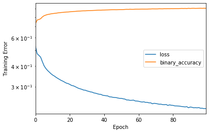
Wrapping up
The MLP version of collaborative filtering shows very promising result compared to the classical matrix factorization. In the future post, we will fuse the two models, i.e. MF and MLP, into a hybrid one, also known as Neural Collaborative Filtering.
