
If you are human and curious about your future, then the recurrent neural network (RNN) is definitely a tool to consider. Part 1 will demonstrate some simple RNNs using TensorFlow 2.0 and Keras functional API.
What is RNN
An RNN is a class of artificial neural networks where connections between nodes form a directed graph along a temporal sequence (time series). This allows it to exhibit temporal dynamic behaviour.
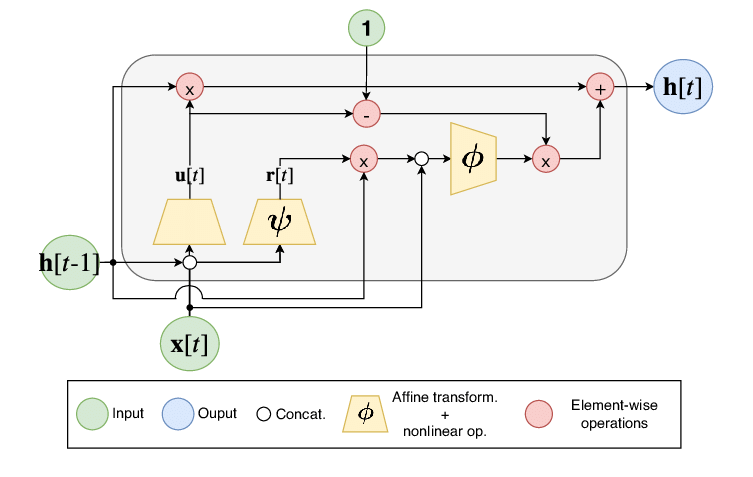
RNNs come in many variants, such as fully recurrent, Elman networks and Jordan networks, Long short-term memory, Bi-directional, etc. Nevertheless, the basic idea of RNN is to memory patterns from the past using cells to predict the future.
The time-series data
In this demo, we first generate a time series of data using a sinus function. We then fetch the data into an RNN model for training and then get some prediction data.
First, we enable TensorFlow 2.0 and import some libraries
%tensorflow_version 2.x
import numpy as np
import tensorflow as tf
import tensorflow.keras as keras
import matplotlib as mpl
import matplotlib.pyplot as plt
%matplotlib inline
The data follows the simple equation:

 where
where 
The following function generates time-series data following above equation.
def generate_time_series(batch_size, n_steps):
    freq1, offsets1 = np.random.rand(2, batch_size, 1)
    time = np.linspace(0, 1, n_steps)
    series = 0.5 * np.sin((time - offsets1) * (freq1 * 10 + 10))  #   sine wave
    return series[..., np.newaxis].astype(np.float32)
We want to generate the train, validation, and test data where every n_steps (n data points) we have one next value (one step ahead for t+1) (see Figure 2).
n_steps = 50
#generate 10k data points
series = generate_time_series(10000, n_steps + 1)
X_train, y_train = series[:7000, :n_steps], series[:7000, -1]
X_valid, y_valid = series[7000:9000, :n_steps], series[7000:9000, -1]
X_test, y_test = series[9000:, :n_steps], series[9000:, -1]
The shapes of x_train and y_train:
X_train.shape, y_train.shape
#((7000, 50, 1), (7000, 1))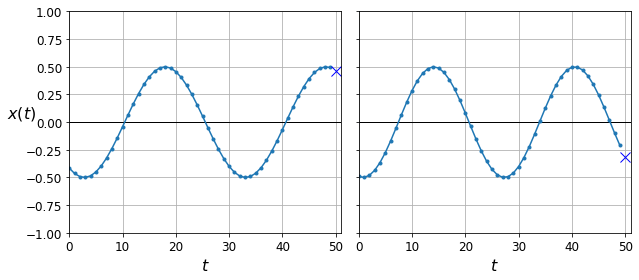
.) from 0-> 50, we have one point (X) at (t+1)Prediction with the simplest RNN
With Keras, things can be very pretty straightforward. We will first try with a shallow RNN with only one layer.
model = keras.models.Sequential([
    keras.layers.SimpleRNN(1, input_shape=[None, 1])
])
That is it, then we compile the model using Adam optimizer.
optimizer = keras.optimizers.Adam(lr=0.005)
model.compile(loss="mse", optimizer=optimizer)
After that, we train the model and log the mean squared error each epoch.
history = model.fit(X_train, y_train, epochs=20, validation_data=(X_valid, y_valid))Remember that, if you don’t pass validation data, then you won’t have val_loss in history. Now, we can plot the training loss using the flowing function:
def plot_learning_curves(loss, val_loss):
    plt.plot(np.arange(len(loss)) + 0.5, loss, "b.-", label="Training loss")
    plt.plot(np.arange(len(val_loss)) + 1, val_loss, "r.-", label="Validation loss")
    plt.gca().xaxis.set_major_locator(mpl.ticker.MaxNLocator(integer=True))
    plt.axis([1, 20, 0, 0.05])
    plt.legend(fontsize=14)
    plt.xlabel("Epochs")
    plt.ylabel("Loss")
    plt.grid(True)
plot_learning_curves(history.history["loss"], history.history["val_loss"])
plt.show()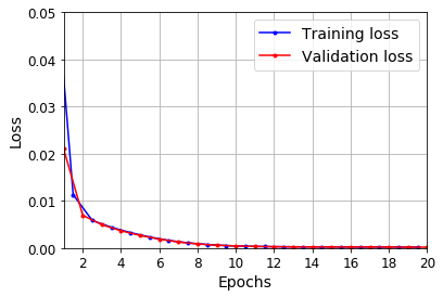
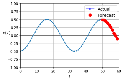
Predict on validation data and plot the result (the last point on the series):
y_pred = model.predict(X_valid)
plot_series(X_valid[0, :, 0], y_valid[0, 0], y_pred[0, 0])
plt.show()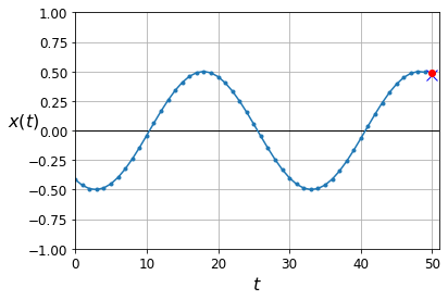
o) VS Validation(bluex)Forecasting several steps ahead
This is the fun part to predict some more steps in the future (so you don’t have to go to a foreteller :D). First, we generate new data.
series = generate_time_series(1, n_steps + 30)
X_new, Y_new = series[:, :n_steps], series[:, n_steps:]
X = X_new
Next, we will predict 30 steps ahead ( ) one by one.
for step_ahead in range(30):
    y_pred_one = model.predict(X[:, step_ahead:])[:, np.newaxis, :]
    X = np.concatenate([X, y_pred_one], axis=1)
Y_pred = X[:, n_steps:]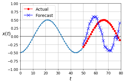
As shown in Figure 3, the accuracy is not really good with one-by-one prediction. Now we can modify the model so that it can predict several at once. The new model supports 10 steps ahead at once:
model = keras.models.Sequential([
    keras.layers.SimpleRNN(20, return_sequences=True, input_shape=[None, 1]),
    keras.layers.SimpleRNN(20),
    keras.layers.Dense(10)
])
We then see a better result with this model.
Note on replacing outputprojectionwrapper from TF1.X
If you work with TensorFlow 1.X, there is a good chance that you use OUTPUTPROJECTIONWRAPPER for your RNN model.

Unfortunately, this function was deprecated in TF2.0 and was not included in the tf.compat.v1. A dense layer is recommended for that based on this post. Therefore, I include another example for ones who want to convert their model from TF1.x to TF2.x. We simply stack up another dense layer at the end (similar to the previous example).
model = keras.models.Sequential([
    keras.layers.SimpleRNN(20, return_sequences=True, input_shape=[None, 1]),
    keras.layers.Dense(1)
])
Conclusion
Working with a recurrent neural network is fun. Nevertheless, the current setting did not fully exploit the power of the RNN. The next part, we will create more complicated data and apply with deeper models of RNN and different cell types, such as LSTM or GRU.

[…] In part 1, we introduced a simple RNN for time-series data. To continue, this article applies a deep version of RNN on a real dataset to predict monthly milk production. […]