deep learning: Linear Autoencoder with Keras

This post introduces using linear autoencoder for dimensionality reduction using TensorFlow and Keras.

What is a linear autoencoder

An autoencoder is a type of artificial neural network used to learn efficient data codings in an unsupervised manner. The aim of an autoencoder is to learn a representation (encoding) for a set of data, typically for dimensionality reduction, by training the network to ignore signal “noise”.

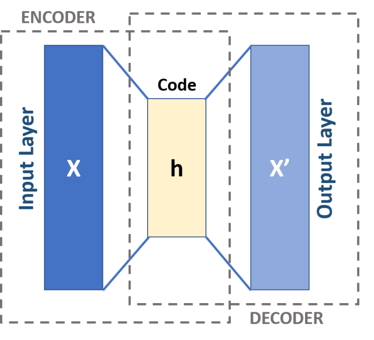
Autoencoders consists of two main parts: encoder and decoder (figure 1). They work by automatically encoding data based on input values, then performing an activation function, and finally decoding the data for output. A bottleneck (the h layer(s)) of some sort imposed on the input features, compressing them into fewer categories. Thus, if some inherent structure exists within the data, the autoencoder model will identify and leverage it to get the output.

A linear autoencoder uses zero or more linear activation function in its layers.

other variations

• Denoising AutoEncoders: Another regularization technique in which we take a modified version of our input values with some of our input values turned in to 0 randomly.
• Sparse AutoEncoders: Where the hidden layer is greater than the input layer but a regularization technique is applied to reduce overfitting. Adds a constraint on the loss function, preventing the autoencoder from using all its nodes at a time.
• Contractive AutoEncoders: Adds a penalty to the loss function to prevent overfitting and copying of values when the hidden layer is greater than the input layer.
• Stacked AutoEncoders: When you add another hidden layer, you get a stacked autoencoder. It has 2 stages of encoding and 1 stage of decoding.

When to use

• Dimensionality reduction/Feature detection
• Building powerful recommendation systems
• Encoding features in massive datasets

Note that: Under a certain circumstance, the solutions for linear autoencoders are those provided by PCA. We will cover PCA in another post. For an encoder on graph data, follow this link.

example with Keras and TF.2.x

We first generate two-class data with 3 dimensions. Then we will use a linear autoencoder to encode (compress) the input data into 2-dimensional data.

import numpy as np
import matplotlib.pyplot as plt
%matplotlib inline
%tensorflow_version 2.x
import tensorflow as tf
from tensorflow.keras.layers import Input, Dense
from tensorflow.keras.models import Sequential

The data is generated by sklearn.datasets.

from sklearn.datasets import make_blobs
data = make_blobs(n_samples=100, n_features=3, centers=2, random_state=101)

We now process data with a minmaxscaler. For each value in a feature, MinMaxScaler subtracts the minimum value in the feature and then divides by the range. The range is the difference between the original maximum and original minimum.

from sklearn.preprocessing import MinMaxScaler
scaler = MinMaxScaler()
scaled_data = scaler.fit_transform(data[0])#only the data (not the labels)

Now, we plot the data:

from mpl_toolkits.mplot3d import Axes3D
fig = plt.figure()
ax = fig.add_subplot(111, projection='3d')
data_x = scaled_data[:,0]#col 1
data_y = scaled_data[:,1]#col 2
data_z = scaled_data[:,2]#col 3
ax.scatter(data_x, data_y, data_z, c=data[1])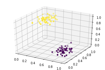

Build an autoencoder model

num_inputs = 3 #input dimensions
num_hidden = 2 #output dimensions in hidden layer h
num_outputs = num_inputs #output and input have the same dim

Next, we build the model from the defined parameters. As this is a linear one, we don’t use any activation function.

inputs = Input(num_inputs)
hidden = Dense(num_hidden)
outputs = Dense(num_outputs)
model = Sequential([inputs,hidden, outputs], name='autoencoder')
optimizer = tf.keras.optimizers.Adam(learning_rate)
model.compile(optimizer=optimizer, loss='mean_squared_error', metrics=['mse'])
model.summary()

Model: "encoder"
_________________________________________________________________
Layer (type)                 Output Shape              Param #
=================================================================
dense_15 (Dense)             (None, 2)                 8
_________________________________________________________________
dense_16 (Dense)             (None, 3)                 9
=================================================================
Total params: 17
Trainable params: 17
Non-trainable params: 0

Train the model

history = model.fit(x=scaled_data, y=scaled_data, epochs=1000, verbose=False)
plt.plot(history.history['loss'], 'r-', label='loss')
plt.plot(history.history['mse'], 'bo', label='mse')
plt.legend()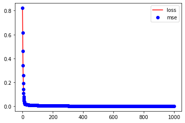

Get the encoded data

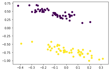
After training, now we can pass the data and get the output from the encoder or the output of the hidden layer.

encoded = hidden(scaled_data)
encoded.shape
#TensorShape([100, 2])

We can see that the output of the hidden layer has only 2 dimensions. Now we can check if the data is still linearly separable after dimensionality reduction.

plt.scatter(encoded[:,0], encoded[:,1], c=data[1])